PhyloSift Tutorial – PE-Illumina data

Here we present an overview tutorial of using PhyloSift with test data consisting of raw, paired-end Illumina Reads

Introduction

PhyloSift can be run using any biological sequence (nucleotide or amino acid). For metagenomes or marker gene studies (e.g. 16S/18S rRNA), you may consider preprocessing steps such as contig assembly or OTU clustering. There are some advantages to this:

• Longer input sequences may improve hits to marker genes, leading to better taxonomy assignments
• Preprocessing substantially reduces the number of input sequences, and may noticeably reduce computational time.
• Datasets can be streamlined by filtering out non-target sequences such as vectors or contaminants. This may lead to greater clarity in your taxonomic results.

However, the drawbacks to this include

• Loss of abundance information. However, we have been working closely with the metAMOS software development team and it is possible to import abundance information into PhyloSift if you carry out assemblies within the metAMOS pipeline.

Core Markers vs. Extended Markers

Users can run PhyloSift with different sets of markers, depending on their specific data analysis needs:

1. The Core Marker Set, which is automatically downloaded when running Phylosift using the standard “all” command. The core marker set currently contains ~40 three-domain protein coding genes (DNGNGWU markers), single-copy eukaryote-specific nuclear orthologs, ribosomal RNA genes (16S/18S), mitochondrial genes (mtDNA markers), and plastid and viral markers identified through Markov-clustering algorithms applied to genome datasets.
2. The Extended Marker Set, which is downloaded when users specify the –extended flag. Note that this marker set is an EXTREMELY LARGE download (several Gigabytes in size) but may result in improved taxonomy assignments (more fine-scale assignments at lower taxonomic levels).
3. A Custom Marker Set can be applied when users specify a custom marker file according to the –custom <file> flag, enabling added flexibility within PhyloSift. For example, if you wanted did not want to consider plastid DNA in your metagenome analysis, uploading a custom file containing all marker names except plastid marker packages (folder names as listed in the /share/phylosift/markers directory) will exclude these marker genes from PhyloSift searches.

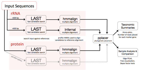
 In this tutorial, we’ll be running through the entire PhyloSift client workflow (all mode as executed using the phylosift wrapper script). A schematic diagram of this workflow is as follows (click to enlarge this image in a new window):

---

PhyloSift Tutorial using Illumina Human Microbiome Data

Step 1: Download and unzip PhyloSift

The latest, stable packaged version of PhyloSift should be downloaded at:

http://edhar.genomecenter.ucdavis.edu/~koadman/phylosift/releases/phylosift_v1.0.1.tar.bz2

Unzip this file within a Finder/Explorer window, or alternatively navigate to the directory where you downloaded the software and run the command:

tar -xvf phylosift_v1.0.1.tar.bz2

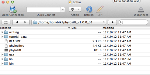
PhyloSift comes prepacked with all the necessary software, and is ready to use once unzipped. After downloading and unpacking the most recent version of PhyloSift from the website, you will see a folder named phylosift_v1.0.1 (note: screenshots below may not reflect the current stable release version; unless otherwise noted, only the top level PhyloSift directory will be different e.g. the phylosift_v1.0.0_* folder)

On the command line, the unzipped folder should appear as:

In a Finder Window (e.g. a server accessed via programs such as CyberDuck, or on your local desktop), the folder will appear as follows:

Step 2: Locate and run Illumina Human Microbiome test data

You’ll notice that the PhyloSift download includes a folder called tutorial_data. All files in this folder were generated from SRA dataset SRX019704, representing Human Microbiome Illumina Paired-end libraries (http://www.ncbi.nlm.nih.gov/sra/?term=SRX019704). For tutorial purposes, we’ve subsampled this HMP Illumina data and provided it to PhyloSift users as a small test dataset consisting of Paired-End Illumina data. This small dataset is comprised of two zipped FASTQ files, HMP_1.fastq.gz and HMP_2.fastq.gz, and these are the input files we’ll be using in this tutorial.

After unzipping PhyloSift, you’ll need to navigate inside the directory (making sure to amend the date extension listed below according to what your downloaded filename is):

cd phylosift_v1.0.1/

Next, execute the following command to run the full PhyloSift workflow (“all” mode) using the HMP test dataset. Note that we will need to specify the –paired flag to indicate PE-Illumina data inputs:

./phylosift all –paired tutorial_data/HMP_1.fastq.gz tutorial_data/HMP_2.fastq.gz

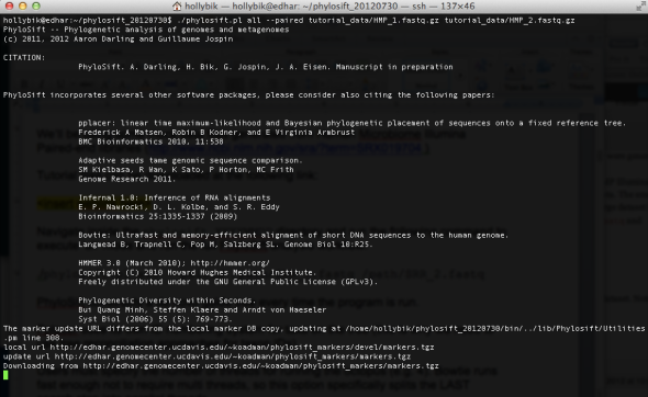
If this command is executed correctly, you will see the following screen:

PhyloSift must first download the latest version of the core marker genes (curated and housed on our UC Davis servers, and provided as an automatic download to users) before processing and analyzing the input data files. The reference marker packages will be downloaded to your home directory (this path will vary depending on your local settings), in the folder /home_directory/share/phylosift/markers/. Note that this directory also contains another folder, /share/phylosift/ncbi/, containing files which are used during tree reconciliation steps (see detailed explanation here) to map NCBI taxon IDs to tree topologies.

Step 3: Explore file outputs from the completed PhyloSift run

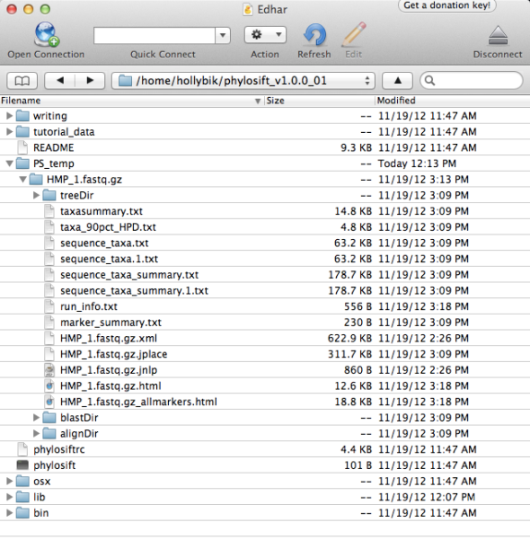
Once the script finishes, you’re ready to explore the results. All results are stored in the directory PS_temp/HMP_1.fastq.gz, which is newly created within your phylosift_v1.0.1 folder. The directory should contain a number of different files and folders, as follows:

Now it’s time to explore the various output files from the PhyloSift workflow. A detailed breakdown of folders and file types can be found here, but in this tutorial we will provide a walk-through of the most relevant file outputs:

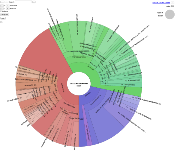
HMP_1.fastq.gz.html, and HMP_1.fastq.gz.allmarkers.html – taxonomy summaries presented in a visual format (presenting the information from the sequence_taxa.txt file). The krona viewer allows dynamic exploration of the data; users can click on a group to expand the taxonomy and view increasingly finer-scale information.

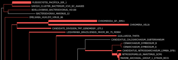
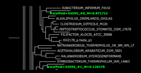
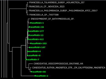
HMP_1.fastq.gz.xml – This file is the fat tree visualization of sequence reads placed on the concat markers (“elite” marker genes, those prefaced by DNGNGWU in the blastDir and alignDir) – it should be viewed using Archaeopteryx tree viewer software packaged in the forester java archive. We automatically convert the concat.jplace file in the treeDir to an XML tree file using the guppy program. Colored branches represent areas where reads were placed, with the thickness of each branch corresponding to the number of reads placed on that branch (see below for example screenshots and more information about tree visualization).

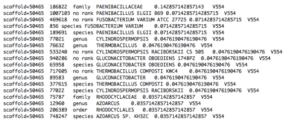
Sequence_taxa_summary.txt – This file contains the raw names of placed samples (for paired samples, both sequences are listed with their FASTQ ids and the suffix /1 or /2) and lists the probability distribution across tree placements. The last column lists the PhyloSift marker packages used to obtain the tree placement for this sequence.

In the best case scenario, a sequence will have 100% probability of being placed at one point on the tree:

Oftentimes, a sequence will show a probability distribution across several different points on the tree, with an obvious “best” placement:

However, the probability distribution for a given sequence may be spread thinly across many parts of the tree, with no obvious “best” placement. Oftentimes this is a function of the reference database, e.g. there may be no sequence data available for a close taxonomic relative within the PhyloSift marker packages, resulting in a “fuzzy” tree placement. In this scenario, the output would look something like this:

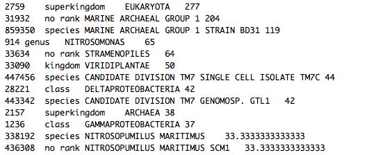
taxa_90pct_HPD.txt, taxasummary.txt – In taxa summary files, the paired info is collated in order to calculate abundance information. One entry is represented for each molecule sequenced.

.jplace files – tree placement file output from pplacer, containing information for read placements and their associatied probability distributions. These files need cannot be explored directly, and first need to be converted using the guppy software tool (see below).

It is important to note that the taxonomic resolution in PhyloSift hinges on the marker packages which are used for analysis. For amino acid alignments, we use a PD pruning approach that reduces taxonomic resolution at genus level and below—amino acid trees are used to infer higher-level phylogenetic placements. For finer taxonomic resolution, we rely on nucleotide alignments and codon subtrees (placement onto clades pruned off of larger trees).

Step 4: Convert .jplace PhyloSift outputs into phylogenetic trees for downstream data visualization and exploration

The guppy software kit (http://matsen.github.com/pplacer/guppy.html) comes prepackaged with PhyloSift in the /phylosift_v1.0.1/bin/ subdirectory. Guppy can be used to convert .jplace output files into tree files (.xml or .tre) which can then be explored in the Archaeopteryx tree viewer (http://www.phylosoft.org/archaeopteryx/)

Fat visualization – outputs trees with colored edges fattened in proportion to the number of reads placed on each branch. (to enable this view, be sure to check ‘colorize branches’ and ‘use branch widths’ in Archaeopteryx)

./guppy fat –out-dir <output directory> pplacer_file.jplace

Example screenshot of a “fat” visualization

Sing visualization- constructs one tree for each placed sequence, enabling users to visualize the probability distributions for each read within the phylogenetic topology.  Since all trees are packaged within one file, we do not recommend the Sing tree visualization unless you are dealing with a small number of placed reads (Archaeopteryx may crash trying to load extremely large files). However, note that it is possible to subsample and/or parse the sing output to view a small number of trees, since each line within the output file contains a different tree. For example, if you are interested in exploring the probability distributions of 5 sequences, you can find these sequences within the text file and pull out the 5 lines (the 5 trees) containing these sequences. This approach avoids the memory limitations with Archaeopteryx .

./guppy sing –out-dir <output directory> pplacer_file.jplace

Example screenshot of a “sing” visualization

Tog visualization – takes the best placement for each sequence read (e.g. location on the tree with the highest posterior probability makes a tree with each of the reads represented as a pendant edge.

 ./guppy tog –out-dir <output directory> pplacer_file.jplace

Example screenshot of a “tog” visualization

---